Neural ODE¤
This example trains a Neural ODE to reproduce a toy dataset of nonlinear oscillators.
This example is available as a Jupyter notebook here.
import time

import diffrax
import equinox as eqx  # https://github.com/patrick-kidger/equinox
import jax
import jax.nn as jnn
import jax.numpy as jnp
import jax.random as jr
import matplotlib.pyplot as plt
import optax  # https://github.com/deepmind/optax
We use Equinox to build neural networks. We use Optax for optimisers (Adam etc.)
Recalling that a neural ODE is defined as
\(y(t) = y(0) + \int_0^t f_\theta(s, y(s)) ds\),
then here we're now about to define the \(f_\theta\) that appears on that right hand side.
class Func(eqx.Module):
    out_scale: jax.Array
    mlp: eqx.nn.MLP

    def __init__(self, data_size, width_size, depth, *, key, **kwargs):
        super().__init__(**kwargs)
        self.out_scale = jnp.array(1.0)
        self.mlp = eqx.nn.MLP(
            in_size=data_size,
            out_size=data_size,
            width_size=width_size,
            depth=depth,
            activation=jnn.softplus,
            final_activation=jax.nn.tanh,
            key=key,
        )

    def __call__(self, t, y, args):
        # Best practice is often to use `learnt_scalar * tanh(MLP(...))` for the
        # vector field.
        return self.out_scale * self.mlp(y)
Here we wrap up the entire ODE solve into a model.
class NeuralODE(eqx.Module):
    func: Func

    def __init__(self, data_size, width_size, depth, *, key, **kwargs):
        super().__init__(**kwargs)
        self.func = Func(data_size, width_size, depth, key=key)

    def __call__(self, ts, y0):
        solution = diffrax.diffeqsolve(
            diffrax.ODETerm(self.func),
            diffrax.Tsit5(),
            t0=ts[0],
            t1=ts[-1],
            dt0=ts[1] - ts[0],
            y0=y0,
            stepsize_controller=diffrax.PIDController(rtol=1e-3, atol=1e-6),
            saveat=diffrax.SaveAt(ts=ts),
        )
        return solution.ys
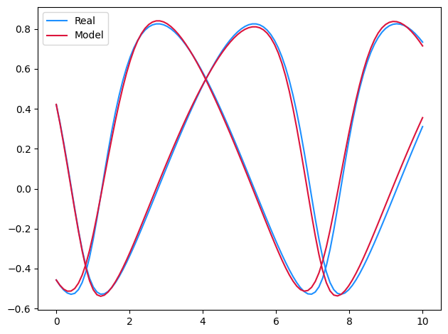
Toy dataset of nonlinear oscillators. Sample paths look like deformed sines and cosines.
def _get_data(ts, *, key):
    y0 = jr.uniform(key, (2,), minval=-0.6, maxval=1)

    def f(t, y, args):
        x = y / (1 + y)
        return jnp.stack([x[1], -x[0]], axis=-1)

    solver = diffrax.Tsit5()
    dt0 = 0.1
    saveat = diffrax.SaveAt(ts=ts)
    sol = diffrax.diffeqsolve(
        diffrax.ODETerm(f), solver, ts[0], ts[-1], dt0, y0, saveat=saveat
    )
    ys = sol.ys
    return ys


def get_data(dataset_size, *, key):
    ts = jnp.linspace(0, 10, 100)
    key = jr.split(key, dataset_size)
    ys = jax.vmap(lambda key: _get_data(ts, key=key))(key)
    return ts, ys
def dataloader(arrays, batch_size, *, key):
    dataset_size = arrays[0].shape[0]
    assert all(array.shape[0] == dataset_size for array in arrays)
    indices = jnp.arange(dataset_size)
    while True:
        perm = jr.permutation(key, indices)
        (key,) = jr.split(key, 1)
        start = 0
        end = batch_size
        while end < dataset_size:
            batch_perm = perm[start:end]
            yield tuple(array[batch_perm] for array in arrays)
            start = end
            end = start + batch_size
Main entry point. Try runnning main().
def main(
    dataset_size=256,
    batch_size=32,
    lr=3e-3,
    steps_strategy=(500, 500),
    length_strategy=(0.1, 1),
    width_size=64,
    depth=2,
    seed=5678,
    plot=True,
    print_every=100,
):
    key = jr.PRNGKey(seed)
    data_key, model_key, loader_key = jr.split(key, 3)

    ts, ys = get_data(dataset_size, key=data_key)
    _, length_size, data_size = ys.shape

    model = NeuralODE(data_size, width_size, depth, key=model_key)
    optim = optax.adabelief(lr)

    # Training loop like normal.
    #
    # Only thing to notice is that up until step 500 we train on only the first 10% of
    # each time series. This is a standard trick to avoid getting caught in a local
    # minimum.

    @eqx.filter_value_and_grad
    def grad_loss(model, ti, yi):
        y_pred = jax.vmap(model, in_axes=(None, 0))(ti, yi[:, 0])
        return jnp.mean((yi - y_pred) ** 2)

    @eqx.filter_jit
    def make_step(ti, yi, model, opt_state):
        loss, grads = grad_loss(model, ti, yi)
        updates, opt_state = optim.update(grads, opt_state)
        model = eqx.apply_updates(model, updates)
        return loss, model, opt_state

    for steps, length in zip(steps_strategy, length_strategy):
        opt_state = optim.init(eqx.filter(model, eqx.is_inexact_array))
        _ts = ts[: int(length_size * length)]
        _ys = ys[:, : int(length_size * length)]
        for step, (yi,) in zip(
            range(steps), dataloader((_ys,), batch_size, key=loader_key)
        ):
            start = time.time()
            loss, model, opt_state = make_step(_ts, yi, model, opt_state)
            end = time.time()
            if (step % print_every) == 0 or step == steps - 1:
                print(f"Step: {step}, Loss: {loss}, Computation time: {end - start}")

    if plot:
        plt.plot(ts, ys[0, :, 0], c="dodgerblue", label="Real")
        plt.plot(ts, ys[0, :, 1], c="dodgerblue")
        model_y = model(ts, ys[0, 0])
        plt.plot(ts, model_y[:, 0], c="crimson", label="Model")
        plt.plot(ts, model_y[:, 1], c="crimson")
        plt.legend()
        plt.tight_layout()
        plt.savefig("neural_ode.png")
        plt.show()

    return ts, ys, model
ts, ys, model = main()
Step: 0, Loss: 0.15854649245738983, Computation time: 2.1308090686798096
Step: 100, Loss: 0.008659855462610722, Computation time: 0.0057790279388427734
Step: 200, Loss: 0.012714792974293232, Computation time: 0.006920814514160156
Step: 300, Loss: 0.009628010913729668, Computation time: 0.007491111755371094
Step: 400, Loss: 0.004102183040231466, Computation time: 0.007421970367431641
Step: 499, Loss: 0.0012518921867012978, Computation time: 0.007432222366333008
Step: 0, Loss: 0.05192319303750992, Computation time: 2.066265106201172
Step: 100, Loss: 0.0171516016125679, Computation time: 0.03773188591003418
Step: 200, Loss: 0.010207891464233398, Computation time: 0.03768420219421387
Step: 300, Loss: 0.01183586660772562, Computation time: 0.04127621650695801
Step: 400, Loss: 0.006402525119483471, Computation time: 0.03928399085998535
Step: 499, Loss: 0.002007006434723735, Computation time: 0.039736032485961914
Some notes on speed: The hyperparameters for the above example haven't really been optimised. Try experimenting with them to see how much faster you can make this example run. There's lots of things you can try tweaking:
- The size of the neural network.
- The numerical solver.
- The step size controller, including both its step size and its tolerances.
- The length of the dataset. (Do you really need to use all of a time series every time?)
- Batch size, learning rate, choice of optimiser.
- ... etc.!
Some notes on being Markov:
- This example has assumed that the problem is Markov. Essentially, that the data
ysis a complete observation of the system, and that we're not missing any channels. Note how the result of our model is evolving in data space. This is unlike e.g. an RNN, which has hidden state, and a linear map from hidden state to data. - If we wanted we could generalise this to the non-Markov case: inside
NeuralODE, project the initial condition into some high-dimensional latent space, do the ODE solve there, then take a linear map to get the output. See the Latent ODE example for an example doing this as part of a generative model; also see Augmented Neural ODEs for a short paper on it.