Step size controllers

The list of step size controllers is as follows. The most common cases are fixed step sizes with diffrax.ConstantStepSize and adaptive step sizes with diffrax.PIDController.

Warning

To perform adaptive stepping with SDEs requires commutative noise. Note that this commutativity condition is not checked.

Abtract base classes

All of the classes implement the following interface specified by diffrax.AbstractStepSizeController.

The exact details of this interface are only really useful if you're using the Manual stepping interface; otherwise this is all just internal to the library.

diffrax.AbstractStepSizeController

Abstract base class for all step size controllers.

wrap(self, direction: int) -> AbstractStepSizeController abstractmethod

Remakes this step size controller, adding additional information.

Most step size controllers can't be used without first calling wrap to give them the extra information they need.

Arguments:

• direction: Either 1 or -1, indicating whether the integration is going to be performed forwards-in-time or backwards-in-time respectively.

Returns:

A copy of the the step size controller, updated to reflect the additional information.

init(self, terms: PyTree[AbstractTerm], t0: Union[float, int], t1: Union[float, int], y0: PyTree[Shaped[ArrayLike, '?*y'], "Y"], dt0: ~_Dt0, args: PyTree[typing.Any], func: Callable[[PyTree[AbstractTerm], Union[float, int], PyTree[Shaped[ArrayLike, '?*y'], "Y"], PyTree[Any]], PyTree[Shaped[ArrayLike, '?*vf'], "VF"]], error_order: Union[float, int]) -> tuple[Union[float, int], ~_ControllerState] abstractmethod

Determines the size of the first step, and initialise any hidden state for the step size controller.

Arguments: As diffeqsolve.

• func: The value of solver.func.
• error_order: The order of the error estimate. If solving an ODE this will typically be solver.order(). If solving an SDE this will typically be solver.strong_order() + 0.5.

Returns:

A 2-tuple of:

• The endpoint \(\tau\) for the initial first step: the first step will be made over the interval \([t_0, \tau]\). If dt0 is specified (not None) then this is typically t0 + dt0. (Although in principle the step size controller doesn't have to respect this if it doesn't want to.)
• The initial hidden state for the step size controller, which is used the first time adapt_step_size is called.

adapt_step_size(self, t0: Union[float, int], t1: Union[float, int], y0: PyTree[Shaped[ArrayLike, '?*y'], "Y"], y1_candidate: PyTree[Shaped[ArrayLike, '?*y'], "Y"], args: PyTree[typing.Any], y_error: Optional[PyTree[Shaped[ArrayLike, '?*y'], "Y"]], error_order: Union[float, int], controller_state: ~_ControllerState) -> tuple[bool, Union[float, int], Union[float, int], bool, ~_ControllerState, diffrax._solution.RESULTS] abstractmethod

Determines whether to accept or reject the current step, and determines the step size to use on the next step.

Arguments:

• t0: The start of the interval that the current step was just made over.
• t1: The end of the interval that the current step was just made over.
• y0: The value of the solution at t0.
• y1_candidate: The value of the solution at t1, as estimated by the main solver. Only a "candidate" as it is now up to the step size controller to accept or reject it.
• args: Any extra arguments passed to the vector field; as diffrax.diffeqsolve.
• y_error: An estimate of the local truncation error, as calculated by the main solver.
• error_order: The order of y_error. For an ODE this is typically equal to solver.order(); for an SDE this is typically equal to solver.strong_order() + 0.5.
• controller_state: Any evolving state for the step size controller itself, at t0.

Returns:

A tuple of several objects:

• A boolean indicating whether the step was accepted/rejected.
• The time at which the next step is to be started. (Typically equal to the argument t1, but not always -- if there was a vector field discontinuity there then it may be nextafter(t1) instead.)
• The time at which the next step is to finish.
• A boolean indicating whether a discontinuity in the vector field has just been passed. (Which for example some solvers use to recalculate their hidden state; in particular the FSAL property of some Runge--Kutta methods.)
• The value of the step size controller state at t1.
• An integer (corresponding to diffrax.RESULTS) indicating whether the step happened successfully, or if it failed for some reason. (e.g. hitting a minimum allowed step size in the solver.)

diffrax.AbstractAdaptiveStepSizeController (AbstractStepSizeController)

Indicates an adaptive step size controller.

Accepts tolerances rtol and atol. When used in conjunction with an implicit solver (diffrax.AbstractImplicitSolver), then these tolerances will automatically be used as the tolerances for the nonlinear solver passed to the implicit solver, if they are not specified manually.

---

diffrax.ConstantStepSize (AbstractStepSizeController)

Use a constant step size, equal to the dt0 argument of diffrax.diffeqsolve.

diffrax.StepTo (AbstractStepSizeController)

Make steps to just prespecified times.

__init__(self, ts: Any)

Arguments:

• ts: The times to step to. Must be an increasing/decreasing sequence of times between the t0 and t1 (inclusive) passed to diffrax.diffeqsolve. Correctness of ts with respect to t0 and t1 as well as its monotonicity is checked by the implementation.

diffrax.PIDController (AbstractAdaptiveStepSizeController)

Adapts the step size to produce a solution accurate to a given tolerance. The tolerance is calculated as atol + rtol * y for the evolving solution y.

Steps are adapted using a PID controller.

Choosing tolerances

The choice of rtol and atol are used to determine how accurately you would like the numerical approximation to your equation.

Typically this is something you already know; or alternatively something for which you try a few different values of rtol and atol until you are getting good enough solutions.

If you're not sure, then a good default for easy ("non-stiff") problems is often something like rtol=1e-3, atol=1e-6. When more accurate solutions are required then something like rtol=1e-7, atol=1e-9 are typical (along with using float64 instead of float32).

(Note that technically speaking, the meaning of rtol and atol is entirely dependent on the choice of solver. In practice however, most solvers tend to provide similar behaviour for similar values of rtol, atol. As such it is common to refer to solving an equation to specific tolerances, without necessarily stating which solver was used.)

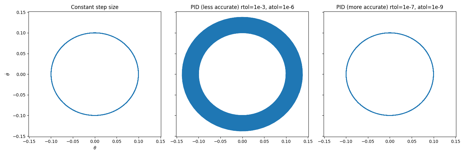
Example

The choice of rtol and atol can have a significant impact on the accuracy of even simple systems. Consider a simple pendulum with a small angle kick:

import diffrax as dfx

def dynamics(t, y, args):
    dtheta = y["omega"]
    domega = - jnp.sin(y["theta"])
    return dict(theta=dtheta, omega=domega)

y0 = dict(theta=0.1, omega=0)
term = dfx.ODETerm(dynamics)
sol = dfx.diffeqsolve(
    term, solver, t0=0, t1=1000, dt0=0.1, y0,
    saveat=dfx.SaveAts(ts=jnp.linspace(0, 1000, 10000),
    max_steps=2**20,
    stepsize_controller=...
)

to compare the effect of different tolerances:

PID_controller_incorrect = diffrax.PIDController(rtol=1e-3, atol=1e-6)
PID_controller_correct = diffrax.PIDController(rtol=1e-7, atol=1e-9)
Constant_controller = diffrax.ConstantStepSize()

The phase portraits of the pendulum from the different tolerances clearly illustrate the impact of the choice of rtol and atol on the accuracy of the solution.

Choosing PID coefficients

This controller can be reduced to any special case (e.g. just a PI controller, or just an I controller) by setting pcoeff, icoeff or dcoeff to zero as appropriate.

For smoothly-varying (i.e. easy to solve) problems then an I controller, or a PI controller with icoeff=1, will often be most efficient.

PIDController(pcoeff=0,   icoeff=1, dcoeff=0)  # default coefficients
PIDController(pcoeff=0.4, icoeff=1, dcoeff=0)

For moderate difficulty problems that may have an error estimate that does not vary smoothly, then a less sensitive controller will often do well. (This includes many mildly stiff problems.) Several different coefficients are suggested in the literature, e.g.

PIDController(pcoeff=0.4, icoeff=0.3, dcoeff=0)
PIDController(pcoeff=0.3, icoeff=0.3, dcoeff=0)
PIDController(pcoeff=0.2, icoeff=0.4, dcoeff=0)

For SDEs (an extreme example of a problem type that does not have smooth behaviour) then an insensitive PI controller is recommended. For example:

PIDController(pcoeff=0.1, icoeff=0.3, dcoeff=0)

The best choice is largely empirical, and problem/solver dependent. For most moderately difficult ODE problems it is recommended to try tuning these coefficients subject to pcoeff>=0.2, icoeff>=0.3, pcoeff + icoeff <= 0.7. You can check the number of steps made via:

sol = diffeqsolve(...)
print(sol.stats["num_steps"])

References

Both the initial step size selection algorithm for ODEs, and the use of an I controller for ODEs, are from Section II.4 of:

@book{hairer2008solving-i,
  address={Berlin},
  author={Hairer, E. and N{\o}rsett, S.P. and Wanner, G.},
  edition={Second Revised Edition},
  publisher={Springer},
  title={{S}olving {O}rdinary {D}ifferential {E}quations {I} {N}onstiff
         {P}roblems},
  year={2008}
}

The use of a PI controller for ODEs are from Section IV.2 of:

@book{hairer2002solving-ii,
  address={Berlin},
  author={Hairer, E. and Wanner, G.},
  edition={Second Revised Edition},
  publisher={Springer},
  title={{S}olving {O}rdinary {D}ifferential {E}quations {II} {S}tiff and
         {D}ifferential-{A}lgebraic {P}roblems},
  year={2002}
}

and Sections 1--3 of:

@article{soderlind2002automatic,
    title={Automatic control and adaptive time-stepping},
    author={Gustaf S{\"o}derlind},
    year={2002},
    journal={Numerical Algorithms},
    volume={31},
    pages={281--310}
}

The use of PID controllers are from:

@article{soderlind2003digital,
    title={{D}igital {F}ilters in {A}daptive {T}ime-{S}tepping,
    author={Gustaf S{\"o}derlind},
    year={2003},
    journal={ACM Transactions on Mathematical Software},
    volume={20},
    number={1},
    pages={1--26}
}

The use of PI and PID controllers for SDEs are from:

@article{burrage2004adaptive,
  title={Adaptive stepsize based on control theory for stochastic
         differential equations},
  journal={Journal of Computational and Applied Mathematics},
  volume={170},
  number={2},
  pages={317--336},
  year={2004},
  doi={https://doi.org/10.1016/j.cam.2004.01.027},
  author={P.M. Burrage and R. Herdiana and K. Burrage},
}

@article{ilie2015adaptive,
  author={Ilie, Silvana and Jackson, Kenneth R. and Enright, Wayne H.},
  title={{A}daptive {T}ime-{S}tepping for the {S}trong {N}umerical {S}olution
         of {S}tochastic {D}ifferential {E}quations},
  year={2015},
  publisher={Springer-Verlag},
  address={Berlin, Heidelberg},
  volume={68},
  number={4},
  doi={https://doi.org/10.1007/s11075-014-9872-6},
  journal={Numer. Algorithms},
  pages={791–-812},
}

__init__(self, rtol: Union[float, int], atol: Union[float, int], pcoeff: Union[float, int] = 0, icoeff: Union[float, int] = 1, dcoeff: Union[float, int] = 0, dtmin: Union[float, int] = None, dtmax: Union[float, int] = None, force_dtmin: bool = True, step_ts: Any = None, jump_ts: Any = None, factormin: Union[float, int] = 0.2, factormax: Union[float, int] = 10.0, norm: Callable[[PyTree], Union[float, int]] = <function rms_norm>, safety: Union[float, int] = 0.9, error_order: Union[float, int] = None)

Arguments:

• rtol: Relative tolerance.
• atol: Absolute tolerance.
• pcoeff: The coefficient of the proportional part of the step size control.
• icoeff: The coefficient of the integral part of the step size control.
• dcoeff: The coefficient of the derivative part of the step size control.
• dtmin: Minimum step size. The step size is either clipped to this value, or an error raised if the step size decreases below this, depending on force_dtmin.
• dtmax: Maximum step size; the step size is clipped to this value.
• force_dtmin: How to handle the step size hitting the minimum. If True then the step size is clipped to dtmin. If False then the differential equation solve halts with an error.
• step_ts: Denotes extra times that must be stepped to.
• jump_ts: Denotes extra times that must be stepped to, and at which the vector field has a known discontinuity. (This is used to force FSAL solvers so re-evaluate the vector field.)
• factormin: Minimum amount a step size can be decreased relative to the previous step.
• factormax: Maximum amount a step size can be increased relative to the previous step.
• norm: A function PyTree -> Scalar used in the error control. Precisely, step sizes are chosen so that norm(error / (atol + rtol * y)) is approximately one.
• safety: Multiplicative safety factor.
• error_order: Optional. The order of the error estimate for the solver. Can be used to override the error order determined automatically, if extra structure is known about this particular problem. (Typically when solving SDEs with known structure.)